My AI Notes - By Ronen Halevy

Building Tensorflow Image Pipeline

Introduction

A Neural Network consists of 2 main components: The Input Data Pipeline and the Network Model.

Having that in mind, a major part in the bring up of any Neural Network, besides setting the model itself, is the setting of an efficient input data pipeline.

The costruction of input data pipeline is an Extract, Transform, Load (ETL) task, so it starts with the extraction of data stored in memory or in files(s), continues with transforming it, such that it will have an efficient data format, and then loading it to the model.

In tensorflow, the data should be extracted and arranged as a tf.data.Dataset object, and then pass through a list of transformations such as decoding batching, normalizing, resizing, shuffling, augmentating, and so forth.

This presents some approaches, each uses a different tf module, for the creation of an image data pipeline. All are alike, in the sense that the output is a tf.data.Dataset object, so all provide an efficient, multiprocessing capeable, yet simple processing forms.

The various data pipeline creation methods are demonstrated over an image classification example - Rock Paper & Scissors.

The source data, Rock Paper Scissors dataset, is listed in TensorFlow Datasets catalog. The dataset was produced by Lawrance Moroney, million thanks for him on that.

The Image Data Pipeline Creation Approaches

This post reviewes 4 approaches:

Using tf.keras.utils module
Using tf.data module
Using tf.keras.preprocessing.image.ImageDataGenerator
Using TFDS module - (which is good only for TensorFlow Datasets)

Arrangement of This Page

In the following we will go step by step through a data classification code, The dataset creation is illustrated using the 4 methods specified above, so the sections which follow are:

Import Packages
Download the data
Create the dataset

3.1 Using tf.keras.utils module

3.2 Using tf.data module

3.3 Using tf.keras.preprocessing.image.ImageDataGenerator

3.4 Using TFDS module

Set the Netowrk Model
Compile the Model
Train
Display Model Summary
Visualize Training Results*
Run Inference

…Here we go…!

1. Import Packages

import tensorflow as tf
import tensorflow_datasets as tfds
import matplotlib.pyplot as plt
import numpy as np
import os
import PIL
from tensorflow import keras
from tensorflow.keras import layers

2. Download the data

Rock Paper Scissors We will use the Rock Paper Scissors dataset, listed in TensorFlow Datasets catalog. The dataset was produced by Lawrance Moroney, million thanks for him on that.

Downloaded Data Format

Here we download the dataset, which is packed as a .zip file.

import pathlib
dataset_name = 'rps'
dataset_url = 'https://storage.googleapis.com/laurencemoroney-blog.appspot.com/rps.zip'
dataset_file = tf.keras.utils.get_file(origin=dataset_url, fname=dataset_name+'.zip', extract=True)

dataset_file point on downloaded file:

print(dataset_file)

/root/.keras/datasets/rps.zip

The downloaded zip file file was extracted , due to the extract=True attribute.

Let’s examine the zip file and the extracted directory:

import os
dataset_dir = pathlib.Path(os.path.dirname(os.path.abspath(dataset_file)))
!ls $dataset_dir

rps  rps-test-set  rps_test.zip  rps.zip

Each dataset subdirectory to a data class: paper rock scissors. Here’s the subdirectory list:

subdir_names = [f for f in os.listdir(os.path.join(dataset_dir, dataset_name))]
print(subdir_names)

['rock', 'scissors', 'paper']

The zip file downloaded so far holds the training data.

The dataset’s author composed another zip file which holds the test data.

Next download it:

dataset_test_name = 'rps_test'
dataset_test_url = 'https://storage.googleapis.com/laurencemoroney-blog.appspot.com/rps-test-set.zip'
dataset_test_file = tf.keras.utils.get_file(origin=dataset_test_url, fname=dataset_test_name+'.zip', extract=True)

!cp -r /root/.keras/datasets/rps-test-set/* /root/.keras/datasets/rps

The train and test datasection are split 80-20. That is fine. but for methodical reasons, The straight forward way to do is to take them as is for training and validation respectively. Methodicaly, we will merge the 2, just to demonstrate the split capabilities of the method which follows in the next notebook cell.

Let’s check how much data have we got by counting number of files in each class directory

from os import listdir
from os.path import isfile, join
import os

class_dir_info = {}
file_ext = 'png'

base_data_dir = os.path.join(dataset_dir, 'rps')
for subdir_name in subdir_names:
  subdir = pathlib.Path(os.path.join(base_data_dir, subdir_name))
  import os, random
  files_count = len([file for file in os.listdir(subdir) if file.endswith(file_ext)])
  class_dir_info.update({'dir': subdir})
  print('{}: {} files'.format(subdir_name, files_count))

print('total file count: {}'.format(len(list(pathlib.Path(base_data_dir).glob('*/*.{}'.format(file_ext))))))

rock: 964 files
scissors: 964 files
paper: 964 files
total file count: 2892

Visualization - take a brief look at randomly selected images from each class

plt.figure(figsize=(15, 15))
for i, subdir_name in enumerate(subdir_names):
  path = pathlib.Path(os.path.join(base_data_dir, subdir_name))
  filename =random.choice(os.listdir(path))
  ax = plt.subplot(1, len(subdir_names), i + 1)
  img = PIL.Image.open(os.path.join(path, filename))
  plt.imshow(img)
  plt.axis("off")
  plt.title(subdir_names[i]+str(img.size))

png

3. Create the Data Pipeline (Extract + Transform)

Having downloaded and extracted the source data files, we we start the creation of data pipeline. So now we demonstrate the various approaches.

Common Parameters consumed by all approaches:

batch_size = 32
image_height = 224
image_width = 224

Each of 3.x paragraphs which follow correspond to a different data pipeline creation approach.

3.1 Create the Data Pipeline Using tf.keras.utils module

This approach uses tf.keras.utils.image_dataset_from_directory method to create the dataset from the source image files.

This is a convinience method, with helpfull features such as:

Option to automatically obtain the data lables according to the subdirectory name, (“inferred” mode).
Transparently supports various image coding formats: : jpeg, png, bmp, gif, where Animated gifs are truncated to the first frame. Accordingly, it is not needed to explicitly decode the images e.g. no need to decode jpeg images.
Supports attributes for data transformation such as batching, shuffling and splitting

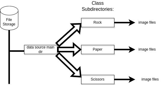
Preliminary Requirements:

For Labels Inferred Mode (which deployed here)- It is assumed that source image files are arranged in subdirectories, each corresponds to a class, as illustrated in the image which follows:

Image Source File Arrangement

Resnet Residual Block

Create training dataset:

train_ds = tf.keras.utils.image_dataset_from_directory(
  directory=base_data_dir, 
  labels="inferred", 
  validation_split=0.2,
  subset="training",
  seed=123,
  image_size=(image_height, image_width),
  shuffle=True, # shuffle is default anyways...
  batch_size=batch_size)

Found 2892 files belonging to 3 classes.
Using 2314 files for training.

Notes on some of the above attributes:

directory: is where the data is located. If labels is “inferred”, it should contain subdirectories, each containing images for a class. Otherwise, the directory structure is ignored

labels=’inferred’ (default). This assumes that the labels are generated from the directory structure.

validation_split: 20% of the dataset is assigned to validation, while the other 80% for training.

subset: This field must be either training or testing. If subset is set, validation_split must be set, and inversely.

batch_size: Default 32

image size Image dimenssions are set to 224x224. (Constraint - each dimenssion should be a multiple of 32, since model contains 5 pooling modules, each downsizes both dimenssions by a factor of 2)

color_mode=rgb (default)

class_names = train_ds.class_names
print(class_names)

['paper', 'rock', 'scissors']

Similarly, create the validation set

val_ds = tf.keras.utils.image_dataset_from_directory(
  directory=base_data_dir, 
  validation_split=0.2,
  subset="validation",
  seed=123,
  image_size=(image_height, image_width),
  batch_size=batch_size)

Found 2892 files belonging to 3 classes.
Using 578 files for validation.

Take some methodical observations:

3.2 Create the Data Pipeline Using tf.data module

3.3 Create the Data Pipeline Using tf.keras.preprocessing.image.ImageDataGenerator

3.4 Create the Data Pipeline Using TFDS module

train_ds.element_spec

(TensorSpec(shape=(None, 224, 224, 3), dtype=tf.float32, name=None),
 TensorSpec(shape=(None,), dtype=tf.int32, name=None))

Examine a single batches shapes:

for image_batch, labels_batch in train_ds.take(1):
  print(image_batch.shape)
  print(labels_batch.shape)
  break

(32, 224, 224, 3)
(32,)

Configure the dataset for performance

The dataset Some data transformations were already defined executed by image_dataset_from_directory. That includes batching, image format decoding, splitting and resizing.

Next we will define more essential transformations:

Dataset.cache keeps the images in memory after they’re loaded off disk during the first epoch.
Dataset.prefetch overlaps data preprocessing and model execution while training. (The tf.data.AUTOTUNE parameter defines a dynamic tuning of the number of prefetched data elements. The number depends on the number of batches consumed in a single step, i.e. on parallelism extent).

Cache, Shuffle (for train data only) and Prefetch:

train_ds = train_ds.cache().shuffle(1000).prefetch(buffer_size=tf.data.AUTOTUNE)
val_ds = val_ds.cache().prefetch(buffer_size=tf.data.AUTOTUNE)

image_batch, label_batch = next(iter(train_ds))

plt.figure(figsize=(10, 10))
for i in range(9):
  ax = plt.subplot(3, 3, i + 1)
  plt.imshow(image_batch[i].numpy().astype("uint8"))
  label = label_batch[i]
  plt.title(class_names[label])
  plt.axis("off")

png

Normalize the data

Standardizes the inputs. This is often integrated within the model, but can also be set on the dataset like so:

normalization_layer = layers.Rescaling(1./255)

train_ds = train_ds.map(lambda x, y: (normalization_layer(x), y))
val_ds = val_ds.map(lambda x, y: (normalization_layer(x), y))

train_ds

<MapDataset shapes: ((None, 224, 224, 3), (None,)), types: (tf.float32, tf.int32)>

Data Augmentation - Expand training dataset size

(Find details on Data Augmentation in a related post (TBD))

data_augmentation = keras.Sequential(
  [
    layers.RandomFlip("horizontal",
                      input_shape=(image_height,
                                  image_width,
                                  3)),
    layers.RandomRotation(0.9, fill_mode="nearest",),
    layers.RandomZoom(0.1),
  ]
)

Demonstrate Augmentation Visualization:

Original image is at upper left, with 8 randomly augmented images.

Note that dataset is exended to be 4 dims, as expected by the augmentation methods.

plt.figure(figsize=(10, 10))
for images, _ in train_ds.take(1):
  image = images[random.randint(0, len(images)-1)]
  ax = plt.subplot(3, 3, 1)
  ax.set_title('original')
  plt.imshow(image)
  ax.set_xticks([])
  ax.set_yticks([])

  for i in range(8):
    augmented_images = data_augmentation((tf.expand_dims(image, axis=0, name=None)))
    ax = plt.subplot(3, 3, i + 2)
    plt.imshow(augmented_images[0].numpy().astype("float32"))
    plt.axis("off")

png

Set Augmentation to training dataset

train_ds = train_ds.map(lambda x, y: (data_augmentation(x), y))

5. Set the model

The model consists of 7 layers:

It begins with 5 convolution blocks, each followed by a max pooling module.
Then, after flattening the data, convolution blocks are followed by 2 dense layers:
A 128 units dense layer
The output layer, with 3 units according to the 3 output classes, i.e.rock, paper, scizors.

num_classes = 3

model = tf.keras.Sequential([
  tf.keras.layers.Conv2D(64, 3, activation='relu', padding='SAME'),
  tf.keras.layers.MaxPooling2D(),
  tf.keras.layers.Conv2D(64, 3, activation='relu', padding='SAME'),
  tf.keras.layers.MaxPooling2D(),
  tf.keras.layers.Conv2D(128, 3, activation='relu', padding='SAME'),
  tf.keras.layers.MaxPooling2D(),
  tf.keras.layers.Conv2D(128, 3, activation='relu', padding='SAME'),
  tf.keras.layers.MaxPooling2D(),
  tf.keras.layers.Conv2D(128, 3, activation='relu', padding='SAME'),
  tf.keras.layers.MaxPooling2D(),
  tf.keras.layers.Flatten(),
  tf.keras.layers.Dropout(0.5),
  tf.keras.layers.Dense(512, activation='relu'),
  tf.keras.layers.Dense(num_classes,  activation = 'softmax')
])

6. Compile the Model

optimizer adam - a commonly used stochastic adaptive optimizer.
loss function SparseCategoricalCrossentropy - commonly used for image classification with more than 2 classes
from_logits=True - This indicate the loss function that that the output is not normalized, i.e. there is no softmax function at the output. BTW, excluding the softmax function from the model, is considered more numerically stable. The softamx is then added by the loss function module.

model.compile(optimizer='adam',
              loss=tf.keras.losses.SparseCategoricalCrossentropy(from_logits=False),
              metrics=['accuracy'])

7. Train the model

Set an Early Stopping Callback

Stop training when a monitored metric has stopped improving.
Wait before stopping according patience value.
Restore best waits, after stopping

early_stop_cb = tf.keras.callbacks.EarlyStopping(monitor='val_loss', 
                                min_delta=0, 
                                patience=10, 
                                verbose=1, 
                                mode='auto', 
                                baseline=None, 
                                restore_best_weights=True)

Now do the fit - 30 epochs, with early_stop_cb.

epochs=30
history = model.fit(
  train_ds,
  validation_data=val_ds,
  epochs=epochs,
  callbacks=[early_stop_cb],
)

Epoch 1/30
73/73 [==============================] - 38s 383ms/step - loss: 1.1026 - accuracy: 0.3224 - val_loss: 1.0581 - val_accuracy: 0.5623
Epoch 2/30
73/73 [==============================] - 26s 362ms/step - loss: 0.9247 - accuracy: 0.5393 - val_loss: 0.7474 - val_accuracy: 0.6401
Epoch 3/30
73/73 [==============================] - 27s 364ms/step - loss: 0.6304 - accuracy: 0.7273 - val_loss: 0.4201 - val_accuracy: 0.8737
Epoch 4/30
73/73 [==============================] - 27s 363ms/step - loss: 0.4464 - accuracy: 0.8181 - val_loss: 0.2478 - val_accuracy: 0.9152
Epoch 5/30
73/73 [==============================] - 27s 366ms/step - loss: 0.2876 - accuracy: 0.8803 - val_loss: 0.2872 - val_accuracy: 0.8875
Epoch 6/30
73/73 [==============================] - 27s 366ms/step - loss: 0.3296 - accuracy: 0.8695 - val_loss: 0.1391 - val_accuracy: 0.9585
Epoch 7/30
73/73 [==============================] - 26s 363ms/step - loss: 0.1646 - accuracy: 0.9395 - val_loss: 0.1666 - val_accuracy: 0.9291
Epoch 8/30
73/73 [==============================] - 26s 361ms/step - loss: 0.1429 - accuracy: 0.9468 - val_loss: 0.1502 - val_accuracy: 0.9325
Epoch 9/30
73/73 [==============================] - 27s 363ms/step - loss: 0.1190 - accuracy: 0.9520 - val_loss: 0.0736 - val_accuracy: 0.9619
Epoch 10/30
73/73 [==============================] - 27s 364ms/step - loss: 0.0925 - accuracy: 0.9693 - val_loss: 0.0771 - val_accuracy: 0.9775
Epoch 11/30
73/73 [==============================] - 27s 367ms/step - loss: 0.0941 - accuracy: 0.9702 - val_loss: 0.0589 - val_accuracy: 0.9775
Epoch 12/30
73/73 [==============================] - 26s 361ms/step - loss: 0.0882 - accuracy: 0.9710 - val_loss: 0.0676 - val_accuracy: 0.9775
Epoch 13/30
73/73 [==============================] - 26s 363ms/step - loss: 0.0764 - accuracy: 0.9715 - val_loss: 0.0625 - val_accuracy: 0.9758
Epoch 14/30
73/73 [==============================] - 26s 362ms/step - loss: 0.0536 - accuracy: 0.9810 - val_loss: 0.0339 - val_accuracy: 0.9896
Epoch 15/30
73/73 [==============================] - 27s 363ms/step - loss: 0.0813 - accuracy: 0.9736 - val_loss: 0.0283 - val_accuracy: 0.9948
Epoch 16/30
73/73 [==============================] - 27s 364ms/step - loss: 0.0415 - accuracy: 0.9875 - val_loss: 0.0146 - val_accuracy: 0.9965
Epoch 17/30
73/73 [==============================] - 27s 363ms/step - loss: 0.0408 - accuracy: 0.9840 - val_loss: 0.0131 - val_accuracy: 0.9948
Epoch 18/30
73/73 [==============================] - 26s 362ms/step - loss: 0.0421 - accuracy: 0.9844 - val_loss: 0.0168 - val_accuracy: 0.9931
Epoch 19/30
73/73 [==============================] - 26s 362ms/step - loss: 0.0663 - accuracy: 0.9801 - val_loss: 0.0149 - val_accuracy: 0.9948
Epoch 20/30
73/73 [==============================] - 26s 360ms/step - loss: 0.0713 - accuracy: 0.9780 - val_loss: 0.0156 - val_accuracy: 0.9948
Epoch 21/30
73/73 [==============================] - 26s 362ms/step - loss: 0.0420 - accuracy: 0.9853 - val_loss: 0.0190 - val_accuracy: 0.9931
Epoch 22/30
73/73 [==============================] - 26s 362ms/step - loss: 0.0485 - accuracy: 0.9827 - val_loss: 0.0170 - val_accuracy: 0.9948
Epoch 23/30
73/73 [==============================] - 26s 365ms/step - loss: 0.0283 - accuracy: 0.9914 - val_loss: 0.0197 - val_accuracy: 0.9965
Epoch 24/30
73/73 [==============================] - 26s 362ms/step - loss: 0.0302 - accuracy: 0.9901 - val_loss: 0.0118 - val_accuracy: 0.9983
Epoch 25/30
73/73 [==============================] - 27s 364ms/step - loss: 0.0196 - accuracy: 0.9927 - val_loss: 0.0054 - val_accuracy: 1.0000
Epoch 26/30
73/73 [==============================] - 26s 363ms/step - loss: 0.0230 - accuracy: 0.9922 - val_loss: 0.0044 - val_accuracy: 1.0000
Epoch 27/30
73/73 [==============================] - 26s 361ms/step - loss: 0.0122 - accuracy: 0.9983 - val_loss: 0.0037 - val_accuracy: 0.9983
Epoch 28/30
73/73 [==============================] - 27s 363ms/step - loss: 0.0299 - accuracy: 0.9883 - val_loss: 0.0140 - val_accuracy: 0.9931
Epoch 29/30
73/73 [==============================] - 26s 361ms/step - loss: 0.0374 - accuracy: 0.9857 - val_loss: 0.0256 - val_accuracy: 0.9913
Epoch 30/30
73/73 [==============================] - 27s 363ms/step - loss: 0.0274 - accuracy: 0.9918 - val_loss: 0.0051 - val_accuracy: 0.9965

8. Display model summary

model.summary()

Model: "sequential_1"
_________________________________________________________________
 Layer (type)                Output Shape              Param #   
=================================================================
 conv2d (Conv2D)             (None, 224, 224, 64)      1792      
                                                                 
 max_pooling2d (MaxPooling2D  (None, 112, 112, 64)     0         
 )                                                               
                                                                 
 conv2d_1 (Conv2D)           (None, 112, 112, 64)      36928     
                                                                 
 max_pooling2d_1 (MaxPooling  (None, 56, 56, 64)       0         
 2D)                                                             
                                                                 
 conv2d_2 (Conv2D)           (None, 56, 56, 128)       73856     
                                                                 
 max_pooling2d_2 (MaxPooling  (None, 28, 28, 128)      0         
 2D)                                                             
                                                                 
 conv2d_3 (Conv2D)           (None, 28, 28, 128)       147584    
                                                                 
 max_pooling2d_3 (MaxPooling  (None, 14, 14, 128)      0         
 2D)                                                             
                                                                 
 conv2d_4 (Conv2D)           (None, 14, 14, 128)       147584    
                                                                 
 max_pooling2d_4 (MaxPooling  (None, 7, 7, 128)        0         
 2D)                                                             
                                                                 
 flatten (Flatten)           (None, 6272)              0         
                                                                 
 dropout (Dropout)           (None, 6272)              0         
                                                                 
 dense (Dense)               (None, 512)               3211776   
                                                                 
 dense_1 (Dense)             (None, 3)                 1539      
                                                                 
=================================================================
Total params: 3,621,059
Trainable params: 3,621,059
Non-trainable params: 0
_________________________________________________________________

9 Visualize training results

acc = history.history['accuracy']
val_acc = history.history['val_accuracy']

loss = history.history['loss']
val_loss = history.history['val_loss']

epochs_range = history.epoch

plt.figure(figsize=(8, 8))
plt.subplot(1, 2, 1)
plt.plot(epochs_range, acc, label='Training Accuracy')
plt.plot(epochs_range, val_acc, label='Validation Accuracy')
plt.legend(loc='lower right')
plt.title('Training and Validation Accuracy')

plt.subplot(1, 2, 2)
plt.plot(epochs_range, loss, label='Training Loss')
plt.plot(epochs_range, val_loss, label='Validation Loss')
plt.legend(loc='upper right')
plt.title('Training and Validation Loss')
plt.show()

png

10. Inference

Uppload Kaggle Auth Token

To run the following notebook cells which use Kaggle stored dataset, a kaggle auth token (kaggle.json file) is needed.

If you have already a kaggle.json file, the code in the notebook cell which follows will upload it (click on Choose Files).

If you don’t, you can generate one - click here for a post on setting Kaggle API.

Next, run inference over the trained model

3 inference sessions follow:

The first 2 use a test dataset stored at Kaggle, and the last one runs inference over user’s interactively uploaded images.

To run the first 2, you need to upload a Kaggle token, as explained next.

If you prefer to avoid the token upload, you can skip directly to the notebook cell, titled Run Prediction On Interactively uploaded Images.

from google.colab import files

uploaded = files.upload()
  
# Move kaggle.json into ~/.kaggle:
!mkdir -p ~/.kaggle/ && mv kaggle.json ~/.kaggle/ && chmod 600 ~/.kaggle/kaggle.json

Upload widget is only available when the cell has been executed in the current browser session. Please rerun this cell to enable.

Saving kaggle.json to kaggle.json

Download the test dataset from Kaggle and unzip it

!kaggle datasets download -d ronenhalevy/rps-test
!unzip rps-test.zip

rps-test.zip: Skipping, found more recently modified local copy (use --force to force download)
Archive:  rps-test.zip
  inflating: rps_test/paper/papaer9.jpg  
  inflating: rps_test/paper/papar10.jpg  
  inflating: rps_test/paper/paper-2.jpg  
  inflating: rps_test/paper/paper3.jpg  
  inflating: rps_test/paper/paper6.jpg  
  inflating: rps_test/rock/rock.jpg  
  inflating: rps_test/rock/rock3.jpg  
  inflating: rps_test/rock/rock4.jpg  
  inflating: rps_test/rock/rock5.jpg  
  inflating: rps_test/rock/rock7.jpg  
  inflating: rps_test/rock/rock8.jpg  
  inflating: rps_test/rock/sn-rock.jpg  
  inflating: rps_test/scissors/scisors.jpg  
  inflating: rps_test/scissors/scissors3.jpg  
  inflating: rps_test/scissors/scissors4.jpg  
  inflating: rps_test/scissors/scissors5.jpg  
  inflating: rps_test/scissors/scissors6.jpg  
  inflating: rps_test/scissors/scissors7.jpg  
  inflating: rps_test/scissors/scissors8.jpg  
  inflating: rps_test/scissors/sn-scissors.jpg  

Run Prediction over The Test Dataset

def do_prediction(image_folder):
    class_name=[]
    fig = plt.figure()
    fig.set_figheight(15)
    fig.set_figwidth(15)
    cnt = 0
    for jdx, dir1 in enumerate(os.listdir(image_folder)):
        for idx, file in enumerate(os.listdir(os.path.join(image_folder, dir1))):
            cnt += 1
            ax = fig.add_subplot(6, 6, cnt)
            image= os.path.join(image_folder,dir1, file)
            image = tf.io.read_file(image)
            image = tf.io.decode_jpeg(image, channels=3)
            image = tf.image.resize(image, (image_height,image_width))
            image = tf.cast(image / 255., tf.float32)
            ax.imshow(image)
            image = tf.expand_dims(image, axis=0)
            result=model.predict(tf.stack(image, axis=0))
            ax.set_title("{} {}"
              .format(cnt, class_names[np.argmax(result)])
            )          
            ax.set_xticks([])
            ax.set_yticks([])
    return
img_folder='rps_test'
do_prediction(img_folder)

png

Examine prediction results

Obviously, results with validation dataset were much better.

There are a number of miss-classification results. A larger train dataset would probably bring better preformance, e.g. note that all papers in training dataset have gaps between fingers, and scissors images are different than those of the test dataset.

Find Accuracy and Loss

Run model.evaluate over the test dataset. It calculates loss and accuracy for this data.

test_ds = tf.keras.utils.image_dataset_from_directory(
  'rps_test',
  seed=123,
  image_size=(image_height, image_width),
  batch_size=3)

test_ds = test_ds.map(lambda x, y: (normalization_layer(x), y))

results = model.evaluate(test_ds)

print(f'Test {model.metrics_names[0]}: {results[0]} / Test model.metrics_names[1]: {results[1]}')

Found 20 files belonging to 3 classes.
7/7 [==============================] - 0s 5ms/step - loss: 0.7307 - accuracy: 0.8500
Test loss: 0.7307165861129761 / Test model.metrics_names[1]: 0.8500000238418579

Run Prediction On Interactively uploaded Images

In next notebook cell, you can interactively upload test files(s) and execute inference

  uploaded = files.upload()
  cnt = 0
  for path in uploaded.keys():
    img = tf.io.read_file(path)
    img = tf.io.decode_jpeg(img, channels=3)
    image = tf.image.resize(img, [image_height, image_width])
    image = tf.expand_dims(image, axis=0)
    image = image / 255.0
    cnt = cnt + 1
    fig = plt.figure()
    fig.set_figheight(15)
    fig.set_figwidth(15)

    results = model.predict(image)
    result = results[0]
    ax = fig.add_subplot(6, 6, cnt)
    ax.set_title("{} ".format(class_names[np.argmax(result)]))  
    ax.imshow(img)
    ax.set_xticks([])
    ax.set_yticks([])

Upload widget is only available when the cell has been executed in the current browser session. Please rerun this cell to enable.

Saving papaer9.jpg to papaer9 (3).jpg
Saving papar10.jpg to papar10.jpg

png

This site is open source. Improve this page.