Introduction
The Background for proposing this Neural Network model, was the challenge of implementing deeper CNNs to achieve better classification performance. Deeper CNNs resulted with improved performance. This is valid for a various of computer vision tasks such as recognition, detction, segmentation etc. On the other hand, when getting much deeper, problems such as vanishing/exploding gradients become more significant, with symptoms such as growing errors and accuracy degradation.
In their paper from 2015, “Deep Residual Learning for Image Recognition”, Kaiming He, Xiangyu Zhang, Shaoqing Ren & Jian Sun proposed a model which enables the training very deep networks - the Resnet. The paper demonstrates Resnet-34, Resnet-50, Resnet-101 and Resnet-152, which deploy 34, 50, 101 and 152 parametric layers respectively.
Resnet Functional Description
Resnet building block is called a Residual Block which contains a skip connection, aka a short-cut as depicted in Figure 1 and described next.
Figure 1: Resnet Residual Block

As shown by Figure 1, the skip is added to plain connection just before the Relu module, thus providing nolinearity effect to the sum. Note that each conv element is followed by a back normalization module and a ReLu activation module. Note - the values of the stride s and the down-scale parameter d are discussed later.
A Resnet network stacks Residual Blocks back to back, as illustrated by Figure 2.
Figure 2: Resnet-18

Figure 2 depicts a Resnet-18 CNN, named so for the 18 layers. The last layer is an FC (fully connected) layer, which receives the flatten array of data and outputs N recognition classes through a softmax module. Resnet was evaluatedwith ImageNet 2012 classification dataset that consists 1000 classes.
Bottle-neck Resnet
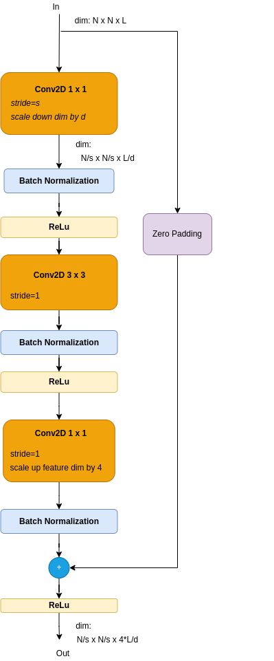
Obviously, yhe deeper the resnet is, the more computation operations are needed - those are counted as FLOPS, where each FLOP is an add/multiply operation. To cope with that, deeper networks, from Resnet50 and up, replace the Resnet Residual block by a Bottlenek Resnet block, as depicted by Figure 3.
Figure 3: Bottlenek Resnet Block
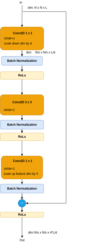
The bottleneck block consists of 3 conv blocks: A single conv 3 x 3, wrapped between 2 conv 1 x 1 blocks. Comparing to the basic Residual Block, this one uses a single conv 3 x 3 module. Note that the conv 3 x 3 requires 9 times more FLOPS than a conv 1 x 1. The conv 3 x 3 is indeed named the bottleneck. The front conv 1 x 1 module scales dimenssions down, to offload the bottleneck, while the conv 1 x 1 scales it up.
Resnet Architectures Table
Table below presents a summerised architecture description of 5 Resnets, presented in the Resnet paper.
Input image size is taken as 224x224 - Anyway, considering the overall image downsizing by 32, both height and width should be a multiple of 32.
The table is copied from the Resnet paper almost as is.
| layer_name | output size | strides | Resnet18 | Resnet34 | Resnet50 | Resnet101 | Resnet152 |
|---|---|---|---|---|---|---|---|
| conv1 | 112x112 | 2 | 7x7,64 | ||||
| conv2.x | 56x56 | 2 | max pool 3x3 | ||||
| 1 or 2 see note (1) | Repeat x2: 3x3,64 3x3,64 |
Repeat x3: 3x3,64 3x3,64 |
Repeat x3: 1x1,64 3x3,64 1x1,256 |
Repeat x3: 3x3,64 3x3,64 3x3,256 |
Repeat x3: 3x3,64 3x3,64 3x3,256 |
||
| conv3.x | 28x28 | 1 or 2 see note (1) |
Repeat x2: 3x3,128 3x3,128 |
Repeat x4: 3x3,128 3x3,128 |
Repeat x4: 1x1,128 3x3,128 1x1,512 |
Repeat x4: 1x1,128 3x3,128 1x1,512 |
Repeat x8: 1x1,128 3x3,128 3x3,512 |
| conv4.x | 14x14 | 1 or 2 see note (1) | Repeat x2: 3x3,256 3x3,256 |
Repeat x6: 3x3,256 3x3,256 |
Repeat x6: 1x1,256 3x3,256 1x1,1024 |
Repeat x23: 1x1,256 3x3,256 1x1,1024 |
Repeat x36: 1x1,256 3x3,256 1x1,1024 |
| conv5.x | 7x7 | 1 or 2 see note (1) | Repeat x2: 3x3,512 3x3,512 |
Repeat x3: 3x3,512 3x3,512 |
Repeat x3: 1x1,512 3x3,512 1x1,2048 |
Repeat x3: 1x1,512 3x3,512 1x1,2048 |
Repeat x3: 1x1,512 3x3,512 1x1,2048 |
FC |
Global average pool, 1000 classes, softmax | ||||||
| 1000 classes + softmax | |||||||
| FLOPS | 1.8x10e9 | 3.6x10e9 | 3.8x10e9 | 7.6x10e9 | 11.3x10e9 | ||
Figure below pillustrates a Resnet-34block diagram.
Figure 4: Resnet-34 block diagram

Dimenssions Matching
The skip connection described above bypassed the processing block directly. This path is known as the Identity Block. However simple, this skip connection may need a dimenssion adaptation to match the direct connection’s dimennsions, if it had been modified. Two methods were proposed to solve that:
- A Skip Block - add extra zero padding to the skip data.
- A Convolutioal block - add a projection 1 x 1 kernel.
Figures below the proposed solutions illustrated on both Residual Block and the Bottleneck Block.
Figure 5a: Residual Block Skip Dimensions Fix with Zero Padding
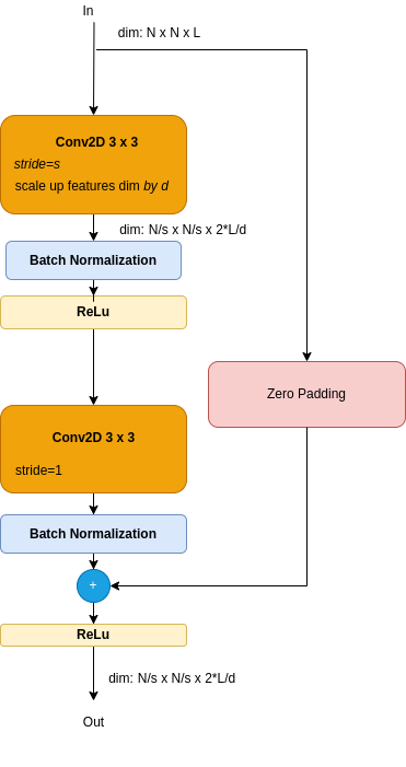
Figure 5b: Residual Block Skip Dimensions Fix with Projection
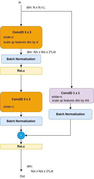
Figure 5c: Bottleneck Skip Dimensions Fix with Zero Padding
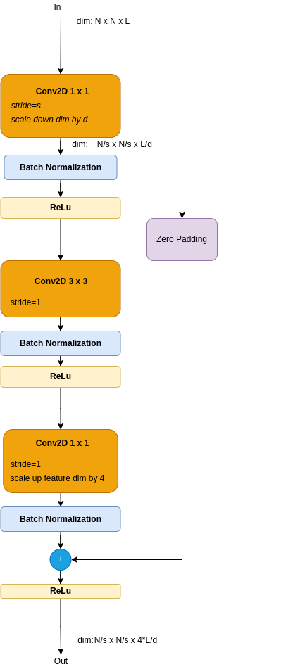
Figure 5c: Bottleneck Skip Dimensions Fix with Projection
Kaiming He et al showed that the projection shortcuts gave better results in terms of top-1 and top-5 error rates (btw, top-5 error rate is the fraction of test images for which none of the five most probable results was the correct lable). On the other hand, padding is needs less coputations, and no extra parameters. The small difference in results made thauthors take the padded skips in their tests, to reduce computation and memory requirements. means that than the simple padding solution.
Considering dimensions matching, here’s a modified Resnet34 block diagram (Figure 4): Now the Residual blocks are indicated as either Identity blockd - or Projection blocks (which could alternatively be Zero Padding blocks).
Figure 6: Resnet-34 block diagram - Indication of Residual blocks types

Notes on Vanishing Gradient problem
A brief reminder of vanishing gradient problem - during the backpropagation, the network’s weights parameters are gradually updated to minimize the loss function, according to Gradient Descent algorithm - or any of its variants.
Here’s the Gradient Descent update equation, for uptating the weights of the kth layer at time \(i+1\):
$w_{i+1}^k=w_i^k+\alpha * \frac{d L}{dw_i^k} $
Where:
- \(w_{i+1}^k\) expresses the kth layer’s weights at time \(i+1\).
- \(\alpha\) is the learning rate
- \(\frac{d L}{dw_i^k}\) is the Loss gradient with respect to the weight at time \(i+1\).
The gradients are calculated using the derivative chain rule, where the optimization calculation is executed in a back propogating manner, starting from layer k=L, back till k=1.
Let’s illustrate the back propogation on a residual block, i.e. the Loss derivative with respect to \(a^{k}\), given \(\frac{dL}{da^{(k+2)}}\).
See Diagram below, which is followed by the xhin rule detivative expression.
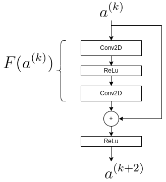
According to chain rule:
\(\frac{dL}{da^{(k)}} = \frac{dL}{da^{(k+2)}}\frac{da^{(k+2)}}{da^{(k)}}\)
Consider that:
\(a^{(k+2)}} = g(F(a^{(k)}) + a^{(k)})
Where g(x) is the activation function, ReLu in this example. ReLu is linear for positive arguments and zero otherwise, so let’s concentrate on the nonw zero case.
In that case, the derivative of the skipped component is 1, so this component protects against vanishing gradient problem.
Besides improving vanishing gradients issue, the skip connections carry lower level information from initial layers which correspnd to lower level features.
Adding this information to the higher level more abstract information extracted by the layers which follow, contributes to better performance.
+Note - check this: https://towardsdatascience.com/understanding-and-coding-a-resnet-in-keras-446d7ff84d33