A Guide To YOLOv3
!!!!!4
Introduction to Object Detection
The task of a CNN object detection model is dual: It provides both classifies objects within an image to dataset labels, and also provides an estimation to objects’ bounding boxes locations. The diagram below illustrates an input image on the left, and classification with bounding box annotations results on the right.
Animation: Image Class and Bounding Box Annotations
A detection model normally outputs 2 vectors per each detected object:
- A Classification output vector, with estimated probabilities of each dataset label. Vector length is \(N_classes\), i.e. number of classes in sdataset. Decision is mostly taken by applying a softmax operator on the vector.
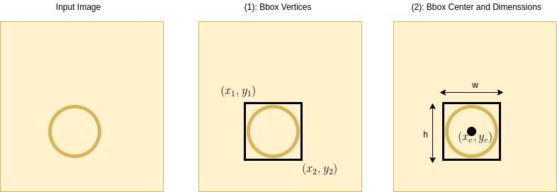
- A vector with the predicted location of a bounding box which encloses the object. The location can be represented in various formats as illustrated in the diagram below.
Representation Formats: (1) Bbox Vertices. (2) Bbox Center + Dimenssions:
Object Detection Models
YOLO was indeed an innovative break-through in the field of CNN Object Detection algorithims. This section briefly reviews 3 object detection algorithms before YOLO.
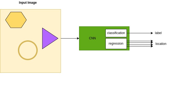
Plain CNN Model
This is a conventional CNN classification model, but classification output stage is now enhanced by a regression predictor for the prediction of a bounding box. Implementation is simple. However, it is limitted to a detection of a single object.
The illustrative diagram which follows presents an image with 3 shape objects. The model, at the best case, will detect one of the object shapes only.
Such detection models, with a detection capability of a sinlge object are often reffered to as Object Localization models.
Figure: Plain CNN Model
Sliding Window Model
To address the single object detectio0n limitation, CNN is repeatedly activated inside the bounderies of a window, as it slides along the image as illustrated in the animation diagram below.
To fit various object sizes, multiple window sizes should be activated, as illustrated in the animation. Alternatively, (or in addition to), the sliding window should run over multiple scaleds of the image.
Location can be determined by window’s region, and the offset of the bounding box within the sliding window position.
Figure: Sliding Window Animation
There are drawbacks to this model: The repeated deployment of the CNN model per each window position, constraints a heavy computation load. But not only that - since convolution span regions are limitted by window’s size and position, which may be uncorrelated with image’s regions of interest postion and sizes, objects may be cropped or missed by the model.
R-CNN
R-CNN (by Ross Girshick et al, UC Berkely, 2014), which stands Regions with CNN features, addresses drawbacks of Sliding Window model.
The idea of R-CNN in essence is of a 3 steps process:
- Extract region proposals - 2000 regions were stated n original paper. The farther process is limitted to proposed regions. There are a number of algorithm which can make region proposals. The authors used selective search by J. Uijlings, K. van de Sande, T. Gevers, and A. Smeulders.Selective search for object recognition.IJCV, 2013.
- Deploy CNN with bounding box regression over each proposed region.
- Classify each region - originally using Linear SVM, in later model’s variants e.g.
Fast R-CNN,Softmaxwas deployed.
Figure: Region Proposals
![alt text]/assets/images/images/yolo/image-classification-rcnn.jpg)
This is just a brief description of the algorithm, which at that time, contributed to a dramatic improvement of CNN detection models performance. R-CNN was later followed by improvments variants such as FASTR-CNN, Girshick, Ross. “Fast r-cnn.” Proceedings of the IEEE international conference on computer vision, 2015, FASTRR-CNN, Shaoqing Ren, Kaiming He, Ross Girshick, Jian Sun, 2016. These models aimed to address R-CNN problems, amongst are real time performance issues,long training time for the 2000 regions and region selection process.
A Brief Introduction to YOLOv3
This article is about YOLO (You Only Look Once), and specifically its 3rd version YOLOv3. YOLOv3: An Incremental Improvement, Joseph Redmon, Ali Farhadi, 2018
As presented above, the common practive in various algorithms prior to YOLO, was to run CNN ver many regions. This ptactices’ computation cost is high.
YOLO does segment the image as well. However, YOLO’s way of segmenting the image is entirely different: instead of running CNN over thousands of regions seperately, it runs CNN only once over the entire image. This is a huge difference, which makes YOLO so much faster - YOLOv3 is 1000 times faster than R-CNN.
So how can YOLO be so fast, while still segmenting the images?
Answer: YOLO functionally segments the image to a grid of cells. But rather than running CNN seperately on each cell, it runs CNN ones.
YOLO’s CNN predicts a detection descriptors to each grid cell. A descriptor combines 2 vectors:
- A Classification result vector which holds a classification probabilty for each of the dataset’s classes.
- The Bounding Box Location $x_1, x1, w, ,h$, along with the Objectness Prediction which indicates probabilty of an object resides in the Bbox.
Animation below illustrates Bounding Boxes parameters, which consist of the center location \(c_x, c_y\), and Width and Height.
Gridded Image Animation: Center location \(c_x, c_y\), Width and Height
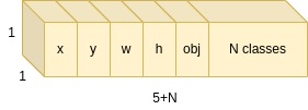
Following is a diagram which illustrates a detection descriptor which YOLO predicts per a detected object. The descriptor consists of 5 words, 4 of which describe the bounding box location, then the Objectness probability, and then N classes probabilities.
Detection Descriptor
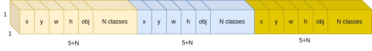
As a matter of fact, YOLOv3 supports not just a single detection per cell, but it supports 3 detections per a cell. Accordingly, YOLO’s predicted descriptor per cell is as illustrated in the diagram below.
Detection 3 Descriptors
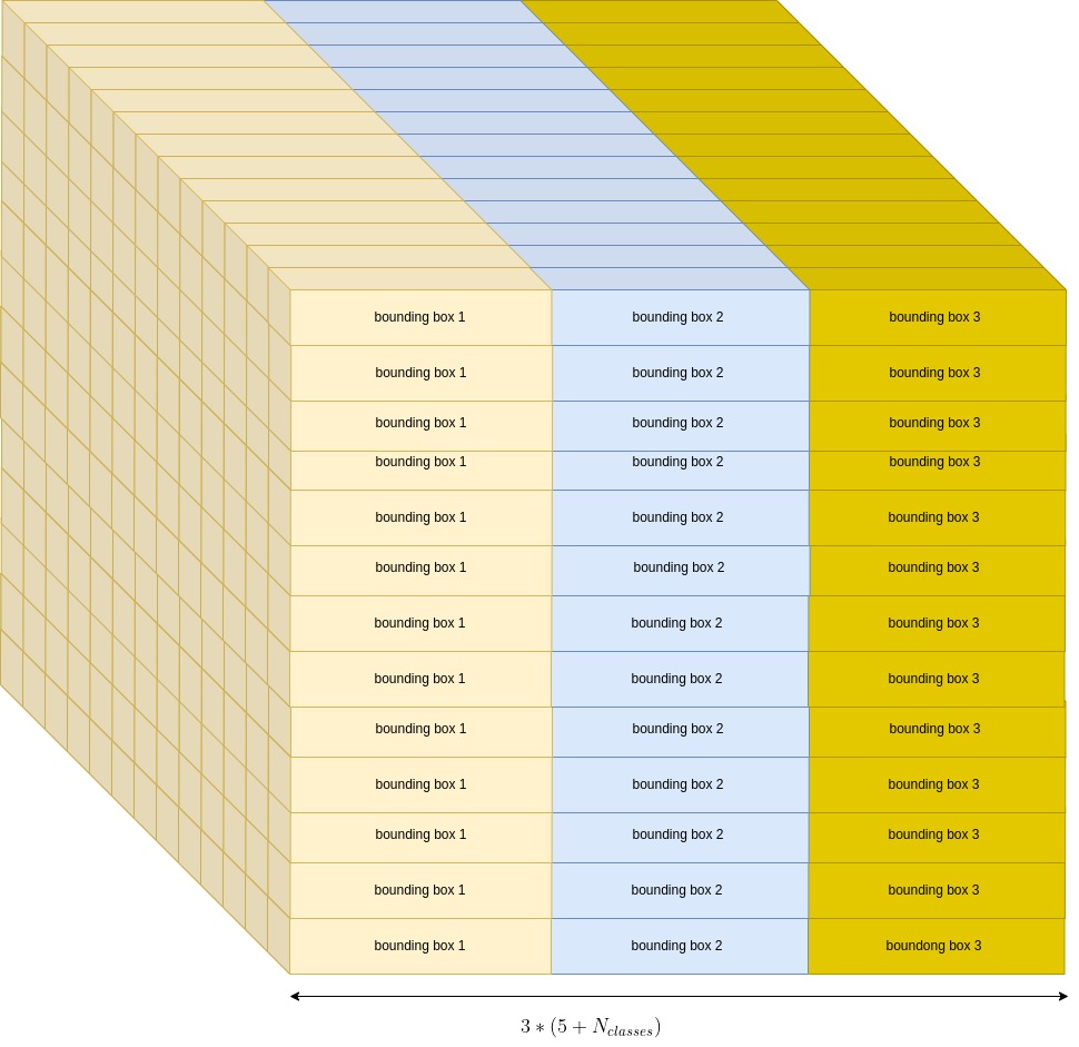
So that was the output for a single grid cell. But CNN assigns such a detection descriptor to each of the grid cells. Considering a 13x13 grid, the CNN output looks like this:
YOLOv3 - CNN Output
Grid Construction
So, how is the grid constructed?
The grid is constructed by passing the image thru a CNN, with a downsampling stride. Image size is 4164163, so assuming a 32 strides downsampling (which is actually the case), the output dimenssions would be a 13 x 13 x N box. Where:
$N=3 x (5+N_{classes})$
That output structure is the illustrated above box diagram.
To enhence detection performance for smaller objects, YOLOv3 CNN generates output in 3 grid scales simultaneously: a 13 x 13 grid (as depicted above), and also 26 x 26 and 52 x 52 grids.
YOLOv3 Block Diagrams
YOLOv3 Block Diagrams
The below block diagrams describe YOLOv3 Forwarding and Training operation.
Following chapters of this article present a detailed description of the 2 operation modes.
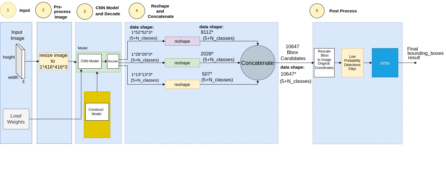
YOLOv3 Block Diagram: Forwarding
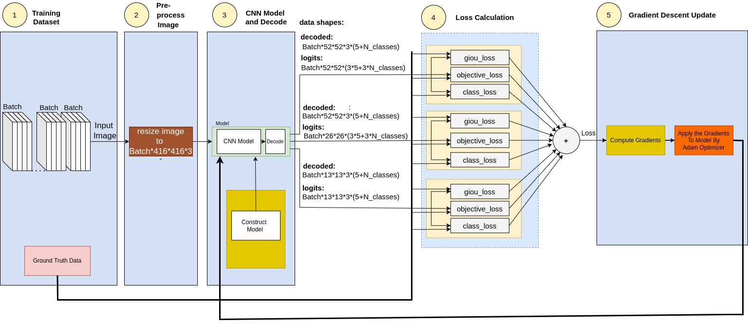
YOLOv3 Block Diagram: Training
The next 2 chapters detail the functionality of Training and Forwarding modes diagrams, following the presented above block diagrams.
YOLOv3 Training Functionality
This section details YOLOv3 Training functionality, following the presented above Training block diagram:
- Training Dataset
- Pre-Process Image
- CNN Model and Decode
- Loss Calculation
- Gradient Descent Update
1. Training Dataset
The training dataset consists of both images examples and their related metadata. The metadata is created per each of the 3 scales. The metadata is arranged to have the same structure like that of the detection descriptor presented in the YOLOv3 introduction section.
For convininence the diagram is posted herebelow again:
Training Arranged Metadata
Let’s illustrate the generation of that metadata with an example:
Herebelow is a training image example:
Training Image Example with Bounding Box Attonations
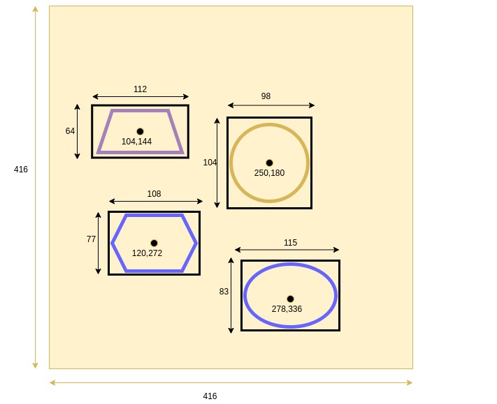
The table below presents the 4 objects’ metadata:
| # | x | y | w | h | Objectness | Class |
|---|---|---|---|---|---|---|
| 1 | 104 | 144 | 112 | 64 | 1 | Trapezoid |
| 2 | 250 | 180 | 98 | 104 | 1 | Circle |
| 3 | 120 | 272 | 108 | 77 | 1 | Hexagon |
| 4 | 278 | 336 | 115 | 83 | 1 | Ellipse |
To construct the training label records, some data arrangements should be taken:
Class Data - Should be arranged as a list of $N_{class}$ priorities. Here $N_{class}$ is 6, since dataset consists of 6 classes: Trapezoid, Circle Heagon, Ellipse, Square and Triangle.
So presentation should be of a one hot format like so:
Trapezoid: 1, 0, 0, 0, 0, 0 Circle: 0, 1, 0, 0, 0, 0 Hexagon: 0, 0, 1, 0, 0, 0 Ellipse: 0, 0, 0, 1, 0, 0
Still, to improve performance, we apply Label Smoothing, as was proposed in Rethinking the Inception Architecture for Computer Visionby Szegedy et al in Rethinking the Inception Architecture for Computer Vision.
| with Label Smmothing, the one-hot probability of y given x, (marked by \((p(y | x) =delta_{y,x}\) ), is smoothed according the formula below: |
Label Smoothing Formula
| \(p_{smoothed}(y | x)=(1-\epsilon)\delta_{y,x}+\epsilon * u(y)\) |
Where:
-
\(\delta(y x)\) is the original one-hot probability - \(\epsilon\) is the smoothing parameter, taken as \(\epsilon=0.01\)
- \(u(y)\) is the distribution over lables, here assumed uniform distribution, i.e. \(u(y)=\frac{1}{6}\).
Pluging the above to Label Smoothing Formula gives:
Objects Class Label Smoothed Probabilities
| p(Trapezoid) | p(Circle) | p(Hexagon) | Ellipse | p(Square) | p(Triangle) | |
|---|---|---|---|---|---|---|
| Trapezoid | 0.990125 | 1.25e-4 | 1.25e-4 | 1.25e-4 | 1.25e-4 | 1.25e-4 |
| Circle | 1.25e-4 | 0.990125 | 1.25e-4 | 1.25e-4 | 1.25e-4 | 1.25e-4 |
| Hexagon | 1.25e-4 | 1.25e-4 | 0.990125 | 1.25e-4 | 1.25e-4 | 1.25e-4 |
| Ellipse | 1.25e-4 | 1.25e-4 | 1.25e-4 | 0.990125 | 1.25e-4 | 1.25e-4 |
The training data is used for loss function computation for the 3 grid scales. To make training data ready for this loss computations, we pack the training labels in 3 label arrays, each relate to a grid scale.
The diagram below shows a 13x13 grid over the image:
Training Image with Anottations with a 13x13 Grid
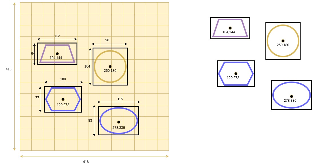
The coarse 13x13 grid diagram shows that the 4 objects are located at cells (3, 4), (7, 5), (3, 8) and (8, 10).
Table below presents the objects related cells per each of the 3 grids.
| #Grid Size | Cell Location Object #1 | Cell Location Object #2 | Cell Location Object #3 | Cell Location Object #4 |
|---|---|---|---|---|
| 13x13 | 3, 4 | 7, 5 | 3, 8 | 8, 10 |
| 26x26 | 6, 8 | 14, 10 | 6, 16 | 16, 20 |
| 52x52 | 12, 16 | 28, 20 | 12, 32 | 32, 40 |
To make training data ready for loss computations, we pack it in 3 label arrays, with shape:
\(\text{labels.shape=Batch} * \text{Grid Size} * N_{boxes} * (5+N_{classes})\)
In our example:
\(\text{coarse-lables.shape=Batch} * 13133 * 11\)
\(\text{medium-lables.shape=Batch} * 26263 * 11\)
\(\text{fine-lables.shape=Batch} * 52523 * 11\)
Now let’s fill in the data to the lable arrays:
coarse-grid lables
The network path to the coarse grid output passes through 32 strides, so accordingly the related grid cells indices are:
index_x1, index_y1 = int(104/32), int(144/32)
index_x2, index_y2 = int(250/32), int(180/32)
index_x3, index_y3 = int(120/32), int(272/32)
index_x4, index_y4 = int(278/32), int(336/32)
index_x1, index_y1 = 3, 4
index_x2, index_y2 = 7, 5
index_x3, index_y3 = 3, 8
index_x4, index_y4 = 8, 10
medium-grid lables
The network path to the coarse grid output passes through 16 strides, so accordingly the related grid cells indices are:
index_x1, index_y1 = 6, 8
index_x2, index_y2 = 14, 10
index_x3, index_y3 = 6, 16
index_x4, index_y4 = 16, 20
fine-grid lables
The network path to the coarse grid output passes through 16 strides, so accordingly the related grid cells indices are:
index_x1, index_y1 = 12, 16
index_x2, index_y2 = 28, 20
index_x3, index_y3 = 12, 32
index_x4, index_y4 = 32, 40
Let Batch=0:
coarse-grid-lables[0,3,4,0,:] =  (0,104,144,112,64,1,0.990125,1.25e-4,1.25e-4,1.25e-4,1.25e-4,1.25e-4)


coarse-grid-lables[0,7,5,0,:] = (0,250,180,98,104,1,0.990125,1.25e-4,1.25e-4,1.25e-4,1.25e-4,1.25e-4)


coarse-grid-lables[0,3,8,0,:] = (0,120,272,108,77,1,0.990125,1.25e-4,1.25e-4,1.25e-4,1.25e-4,1.25e-4)


coarse-grid-lables[0,8,10,0,:] = (0,278,336,115,83,1,0.990125,1.25e-4,1.25e-4,1.25e-4,1.25e-4,1.25e-4)
medium-grid-lables[0,6,8,0,:] =  (0,104,144,112,64,1,0.990125,1.25e-4,1.25e-4,1.25e-4,1.25e-4,1.25e-4)


medium-grid-lables[0,14,10,0,:] = (0,250,180,98,104,1,0.990125,1.25e-4,1.25e-4,1.25e-4,1.25e-4,1.25e-4)


medium-grid-lables[0,6,18,0,:] = (0,120,272,108,77,1,0.990125,1.25e-4,1.25e-4,1.25e-4,1.25e-4,1.25e-4)


medium-grid-lables[0,16,20,0,:] = (0,278,336,115,83,1,0.990125,1.25e-4,1.25e-4,1.25e-4,1.25e-4,1.25e-4)
fine-grid-lables[0,12,16,0,:] =  (0,104,144,112,64,1,0.990125,1.25e-4,1.25e-4,1.25e-4,1.25e-4,1.25e-4)


fine-grid-lables[0,28,20,0,:] = (0,250,180,98,104,1,0.990125,1.25e-4,1.25e-4,1.25e-4,1.25e-4,1.25e-4)


fine-grid-lables[0,12,36,0,:] = (0,120,272,108,77,1,0.990125,1.25e-4,1.25e-4,1.25e-4,1.25e-4,1.25e-4)


fine-grid-lables[0,32,40,0,:] = (0,278,336,115,83,1,0.990125,1.25e-4,1.25e-4,1.25e-4,1.25e-4,1.25e-4)
2. Pre-Process Image
The input images should be resized to 416 x 416 x 3, but preserve the original aspect ratio.
Here’s a pseudo code for image resize. It is followed by an illustrative example.
Note: tf.resize has a preserve_aspect_ratio attribute, so one could consider using it.
    yolo_h, yolo_w    = 416
    orig_h, orig_w _  = image.shape

    scale = min(yolo_w/orig_w, yolo_h/orig_h)
    scaled_w, scaled_h  = int(scale * orig_w), int(scale * orig_h)
    resized_image = np.resize(image, (yolo_w, yolo_h))

    padded_image = np.full(shape=[yolo_h, yolo_w, 3], fill_value=128.0)
    d_w, d_h = (yolo_w - orig_w) // 2, (yolo_h - orig_h) // 2
    padded_image[d_h:orig_h+d_h, d_w:orig_w+d_w, :] = resized_image
Example
Here’s an illustration of the above pseudo code.
Input Image
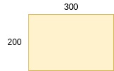
orig_h, orig_w _  = 200, 300

scale = min(416/300, 416/200)
scale = 1.386666667

scaled_w, scaled_h  = int(1.386666667 * 300), int(1.386666667 * 200)
scaled_w, scaled_h  = 416, 277

d_w, d_h = 0, 69
Illustrating Animation
3. CNN Model and Decode
This section presents YOLOv3 CNN, along with its output decoding part, both are parts of the model’s graph.
YOLOv3 CNN is an FCN - A Fully Convolution Network, as it is composed of convolution modules only, without any fully connected component.
The CNN is based on Darknet-53 network as its backbone.
Here below is a high level block scheme of the YOLOv3 CNN. It is followed by a more detailed diagram of same YOLOv3 CNN.
YOLOv3 CNN Hige Level Block Diagram
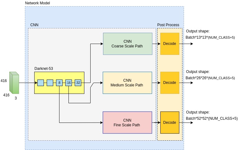
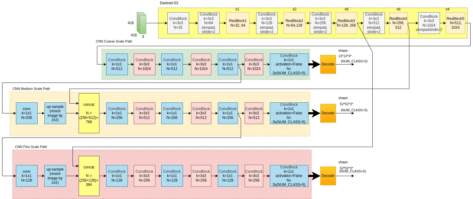
YOLOv3 CNN Detailed Block Diagram
Looking at the above diagrams, one can observe 3 sub-module types:
- Darknet-53, CNN’s backbone.
- Three CNN paths, one per each grid scale
- Decode modules which make a post-process on CNN’s output, before loss function computation.
Next section drills inside the modules, providing detailed insights on architecture.
Darknet-53
Take a look at the Darknet-53 part in the above block diagram and note that:
- Darknet-53 is structured as a cascade of ConvBlocks and ResBlocks.
- The
x1,x2,x8,x4notations on top of the ResNet blocks in the diagram above, indicate of the duplication number of the same module. - Each of the 5 ConvBlocks downsamples by 2 (stride=2), for a total stride 32 at the top stage, and 16 and 8 at the stages before. Those stages feed the coarse, medium and fine scale grids respectively.
Here below is a Block diagrams of ConvBlock. ResBlock follows after.
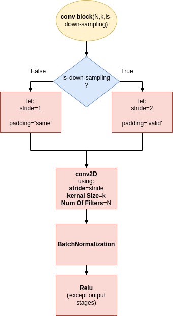
ConvBlock
-
As depicted by the diagram, ConvBlock is a structure which combines a Conv2D module, a BatchNormalization module and a Relu Activation at the top - except for the output stages, where activation is not applied.
-
ConvBlocks have 2 flavors: either with or without downsampling. The downsampling with stride=2 flavor is implemented only within the Darknet-53 block.
-
ConvBlocks’ kernel size is 3 inside Darknet-53, while after that, kernel size alternates between 1 x 1 with N=512 and 3 x 3 with N=1024.
ResBlock
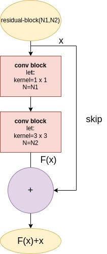
The Res-Block sums up the output of 2 Conv-Blocks with the input data x, aka skipped input.
(If the ResBlocks look familiar - then it indeed is a reuse of the structure presented in the famous ResNet model.
The ResBlock structure provides 2 contributions:
- It helps solving the vanishing gradient problem. (Vanishing Gradient Reminder:, during training back propogation, the gradients are calculated using the chain rule, so a gradient is a multiplication product of previous gradients with its conv block partial derivative. In case the network is deep, gradient values become smaller in layers closer to the top of the network.). since ResBlock’s
skipconnection gradient is unity, the vanishing gradient is prevented. - The mixing of skip layer with the convolutioned layers refines the feature extraction, which benefits from more details provided by the skipped data and features provided by convolutioned layers output.
Why named Darknet-53?
Darknet-53 is because it had 53 layers. However, count of all conv2D elements in Darknet-53, (considering 2 conv2D elements in a ResBlock), sums up to: 1+1+2+1+4+1+16+1+16+1+8=52, not 53.
Still, it had 53 layers, but the fully connected output layer at the top was omitted when deployed in YOLOv3.
3 Scale Paths
YOLOv3 most noticeable improvement wrt earlier YOLOs, was the detection in 3 scales. This improvement enhanced smaller object detection performance, which was a weakness of previous YOLO versions.
As depicted by the above CNN diagram, the 3 scale paths are similarly structured, each with 7 convolution blocks. However, each scale is reduced by a factor of 2 in input data strides and ConvBlocks’ number of filters.
The Concatenation Block
The medium and fine grained paths have an extra Concatenation Block, (See diagram’s 3rd and 4th rows from top). It concatenates data sourced by Darknet-32’s intermidiate stage, together with upsampled data from the preceding scale level path.
Why Concatenating? The concatenation module’s contribution is quite similar to the Res Block’s effect on feature detection refinement. Still, concatenation is applied and not summation, since the 2 datas are sourced by different network stages, which leaves no point for summation.
Decode Module
Decode module is applied on CNN output, namely x,y,w,h,Objectness,Class Priorities, preparing it for Loss Function computation.
Table below summerizes Decode functionality over the data. It is followed by a detailed description of Decode.
| Input | Operation | Output |
|---|---|---|
| x,y | Limit results to 0<=x,y<=1 by applying Sigmoid. Upscale Coordinates to Original Size | x,y, in 416*416 scale |
| w,h | Decode w,h values, Upscale Coordinates to Image Original Size | w,h in 416*416 scale |
| Objectness Probability | Limit value to 0<=Obj<=1 by applying Sigmoid() | 0<=Obj<=1 |
| Class Probabilities | Limit values to 0<=P<=1 by applying Sigmoid() | 0<=Probabilities<=1 |
Decode x,y Coordinates
Let x,y be the CNN predicted values for the location of a bounding box center. Given that x and y, the bounding box center can be computed as presented in the diagram below and in the expression which follows.
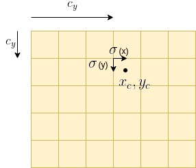
$x_c = c_x + \sigma(x)$
$y_c = c_y + \sigma(y)$
Decode w,h Coordinates
To improve performance of bounding box predicton, YOLOv3 uses anchors for for bounding boxes width and height prediction. An anchor consists of a width and height parameter. YOLOv3 is provisioned with 9 anchor sets, 3 per each scale.
The 9 anchor boxes are generated by performing k-means clustering on the dimensions of the Training data boxes. After that, the 9 anchors are distributed among the 3 scale processes in a decending order - the 3 largest to the coarse scale process and the 3 smallest to the fine scale process.
Accordingly, the CNN does not compute width and height directly, but only parameters for the formula listed below:
-
$w=exp(w)*\textrm{anchor_w}$
-
$h=exp(h)*\textrm{anchor_h}$
BTW, amongst all decoded parameters, only w, h are the not activated by Sigmoid, as their value is restricted to be less equal 1.
Decode Objectness
Objectness holds the probability of an object within the cell. Decode applies a Sigmoid on this parameter, thus confirming value in range 0 <=Objectness <=1
$objectness = sigmoid(objectness)$
Decode Class Probability
Class Probability is also activated by a Sigmoid. Alternatively, a Softmax could be activated, which would require a different Loss Function than we will use here.
$\textrm{class prob} = sigmoid(\textrm{class prob} )$
4. Loss Calculation
Loss Function determines the difference between the expected results and the predicted output. Final objective is to minimize this difference. Thw minimization is produced by an optimization algorithm, which is the next block, covered in the next section.
The overall loss is a sum of all prediction losses, i.e.:
- Bounding Box Prediction Loss
- Objectness Prediction Loss
- Class Prediction Loss
Subsection which follow detail each of the 3.
Bounding Box Prediction Loss
Bounding Box Prediction Loss is dependent on 4 prediction parameters loss, i.e. x,y,w,h. There are various candidates for Loss Functions. Here we will use IOU.
Alternatively, the loss could be taken directly as a sum of x,y,w,h prediction errors like so:
$x_{loss} = \sum_{i=0}^{N_{bbox}}(x^i_{true} - x^i_{predicted})^2$
$y_{loss} = \sum_{i=0}^{N_{bbox}}(y^i_{true} - y^i_{predicted})^2$
$w_{loss} = \sum_{i=0}^{N_{bbox}}(w^i_{true} - w^i_{predicted})^2$
$h_{loss} = \sum_{i=0}^{N_{bbox}}(h^i_{true} - h^i_{predicted})^2$
Where number of bounding boxes is:
$N_{bbox} = BatchSize * GridSize * BoxesInGridCell$
(e.g. For the Coarse Scale Grid, where BatchSize=10, GridSize=13x13, BoxesInGridCell=3, $N_{bbox}=101693=5070$)
But as noted, here we use IOU for Bounding Box Loss calculation.
IOU In Brief: IOU (Intersection over Union) is a term used to describe the extent of overlap of two boxes. The greater the region of overlap, the greater the IOU
IOU is a metric used in object detection benchmarks to evaluate how close the predicted and ground truth bounding boxes are. IOU, as its name indicates, is expressed as the ratio between the intersection area and the union area of the 2 boxes. IOU expression is listed below, followed by an illustrative diagram.
$IOU=\frac{S_{true}\cap S_{pred}}{S_{true} \cup S_{pred}}$
IOU Loss Function
$iou_{loss} = 1 - iou$
Now that IOU is clear, here’s an IOU drawback: it is indifferent for all zero intersection - it is always 0 as illustrated in the diagram below.
IOU Zero Intersection
To overcome this drawback, we introduce GIOUI - a modified IOU algorithm, [Hamid Rezatofighi et al, Generalized Intersection over Union: A Metric and A Loss for Bounding Box Regression](https://arxiv.org/abs/1902.09630.
GIOU
GIOU stands for Generalized IOU. It adds the bounding boxes clossness criteria by considering the difference between the minimal area which encloses the boxes and the boxes union area:
$GIoU=IoU - \frac{S_{enclosed} - {(S_{true} \cup S_{pred})}}{S_{enclosed}}$
Animated diagrams below illustrate $S_{enclosed}$ as a function of boxes clossness.
The final expression used for GIoU Loss adds the consideration of whether there is indeed an object in the cell. This is expressed by $Objectness_{true}$, the ground truth objectness, which value is True if an object indeed exists in the cell, and False otherwise.
$giou_{loss} = Objectness_{true} * (1-giou) $
!!!! RONEN REMOVE GAMA from CODe gives weights to small area!!!!!!!!!!!!!!!!!!!!!!!!!!!!!!!!!!!!!!!!!!!!!!!!1
GIoU Loss - Array Shape
GIoU Loss, same as the 2 other loss functions, is calulated per each bounding box. Accordingly, lose shape is:
- Batch * 13 *13 *3 for coarse grid
- Batch * 26 *26 *3 for medium grid
- Batch * 52 *52f *3 for medium grid
Objectness Prediction Loss
Objectness expresses the probability of an object exisiting in the cell. The Objectness CNN output passes through a Sigmoid activation block - as detailed in the Decoder section of this article.
Consequently, the loss function can be computed by tf.sigmoid_cross_entropy_with_logits():
$\textbf{sigmoid_cross_entropy_with_logits(labels=objectness_true, logits=objectness_pred)}$
The Objectness Loss is ignored in case if there is no object in the cell, but maxIoU (The maximal IoU computed for this cell) is above threshold, i.e. it may indicate of an object.
Table below lists the various states:
| Objectness Ground Truth | maxIoU < IoULossThresh | Objectness Loss |
|---|---|---|
| True | True | Valid |
| True | False | Valid |
| False | True | Valid |
| False | False | Ignore |
Final expression for Objectness Loss:
\(objectness_{loss} = (objectness_{true} +(1.0 - objectness_{true}) * ( maxIoU < IoULossThresh) )* \text{sigmoid_cross_entropy_with_logits}(objectness_{true}, objectness_{pred})\)
Class Prediction Loss
Similar to the Objectness prediction, The classification predictions are also passed through Sigmoid activation - as detailed in the Decoder section.
Consequencly, tf.sigmoid_cross_entropy_with_logits() is used here too as the loss function.
The Classification Loss is ignored if there is no object in the cell i.e.
The Class loss are considered only when Objectness ground true value is True, i.e. there is an object in the cell.
The expression for class loss follows: $objectness_{true} = False$.
So the final expression for Classification Loss is:
$class_{loss} = obj_{true} * \text{sigmoid_cross_entropy_with_logits}(obj_{true}, obj_{pred})$
Classification Loss Shape
Classification Loss, as the 2 other loss functions, is calulated per each bounding box. Accordingly, shape is:
$Classification_{loss}.shape$ = Batch x grid_size x grid_size x 3 x num_of_classes
- Batch * 13 *13 *3 for coarse grid
- Batch * 26 *26 *3 for medium grid
- Batch * 52 *52f *3 for medium grid
The Classification Loss is calulated per each bounding box. The shape is:
- Batch x grid_size x grid_size x 3 x num_of_classes
Where:
grid_size; 13, 26, 52 for coarse, medium and fine grid respectively. num_of_classes: e.g. 80 for coco dataset
Total Loss Function
The total Loss is the sum of all 3 losses in all grid cells, in all 3 grid scales/
total_loss = giou_loss + conf_loss + prob_loss
5.Gradient Descent Update
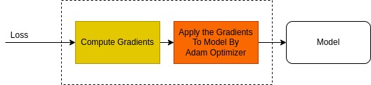
Running Train session under tf.GradientTape ensures the watching of all trainable variables. Following that, the gradient computation and the model update which follows is straight forward.
   with tf.GradientTape() as tape:
        pred_result = model(image_data, training=True)
        total_loss = compute_loss(pred_result, labels)
        gradients = tape.gradient(total_loss, model.trainable_variables)
        optimizer.apply_gradients(zip(gradients, model.trainable_variables))
YOLOv3 Forwarding Functionality
YOLOv3 Forwarding was depicted by the YOLOv3 Forwarding Block Diagram.
Most of the functional blocks are same as detaiiled above Training Mode’s. Still, there is no Loss computation and a Gradient Descent learning mechanism. Instead, weights are either loaded from a file, or were pre-trained before.
The Post Process, marked by #5 in the diagram, is unique to the Forwarding process. Let’s drill into it.
Forwarding Post Process
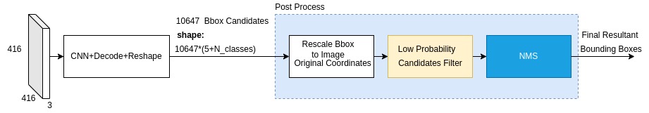
Bounding Boxes Candidates
The Post Processing block selects the final detections amongst all detection candidates it receives. More precisely, select relevant detections amongst the 10647 bounding boxes candidates generated by CNN.
10647 bounding boxes? Let’s show that:
CNN generates 13x13x3 detection descriptor records by the coarse scale path, along with 26x26x3 and 52x52x3 records generated by medium and fine scale CNN paths respectively.
Total number of input records is then:
13x13x3 + 26x26x3 + 52x52x3 = 10647
The structure of each detection descriptor records is illustrated (again) by the diagram below:
Next, these 10647 bounding boxes pass through 2 selection filters:
- Low Probability Candidates Mask
- NMS
These are discussed next.
Rescale Bounding Boxes Coordinates
The bounding box coordinates are rescaled to fit the original image dimenssions.
Let’s illustrate that rescale with an exampe:
Here below is the CNN 416x416 output image, with boundbox annotations arround the ellipse object:
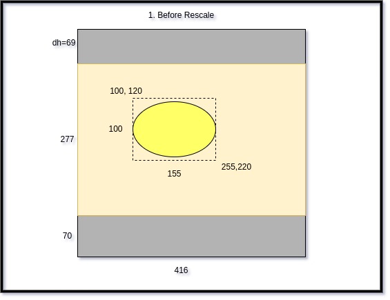
Original dimenssions are 200x300.
The computation of offset shifts and resize ratio are listed below. An anumation illustration follows.
\\(w_{original}, h_{original}= 200,300\\)

\\(resize_ratio = min(\frac{416}{w_{original}}, \frac{416}{h_{original}})\\)

\\(resize_ratio = min(\frac{416}{300}, \frac{416}{200}) = 1.386666667\\)


\\(dh=int((416-resize_ratio*w_{original})/2)=int((416-200*1.386666667)/2)=69\\)
Bbox Rescale Illustration

Low Probability Candidates Filter
This module filters out bbox candidates with low probability, as expressed in the formula below:
scores = pred_conf * class_probability

if scores < score_threshold:
  discard
scores = pred_conf * pred_prob[np.arange(len(pred_coor)), classes] score_mask = scores > score_threshold
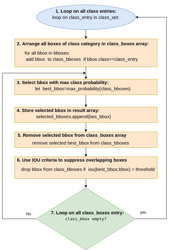
NMS
Non Max Suppression - NMS, aims to remove bounding boxes overlaps. NMS selects bounding boxes with higher predicted class probability, and discards all bounding boxes with same class category, which have a high overlap with theselected boxes. The amount of overlap is metered by IOU.
The algorithm is described in the pseudo code flow chart:
https://towardsdatascience.com/yolo-v3-object-detection-53fb7d3bfe6b#:~:text=More%20bounding%20boxes%20per%20image&text=On%20the%20other%20hand%20YOLO,it’s%20slower%20than%20YOLO%20v2.
https://lilianweng.github.io/lil-log/2017/12/31/object-recognition-for-dummies-part-3.html
https://vivek-yadav.medium.com/part-1-generating-anchor-boxes-for-yolo-like-network-for-vehicle-detection-using-kitti-dataset-b2fe033e5807 : , YOLOv2 does not assume the aspect ratios or shapes of the boxes.
https://machinelearningmastery.com/how-to-perform-object-detection-with-yolov3-in-keras/
http://christopher5106.github.io/object/detectors/2017/08/10/bounding-box-object-detectors-understanding-yolo.html
effectively splits the image into grids of arbitrary size
from https://towardsdatascience.com/yolo-v3-object-detection-53fb7d3bfe6b#:~:text=More%20bounding%20boxes%20per%20image&text=On%20the%20other%20hand%20YOLO,it’s%20slower%20than%20YOLO%20v2. :
YOLO is a fully convolutional network and its eventual output is generated by applying a 1 x 1 kernel on a feature map
https://nico-curti.github.io/NumPyNet/NumPyNet/layers/route_layer.html : Route Layer In the YOLOv3 model, the Route layer is usefull to bring finer grained features in from earlier in the network. This mean that its main function is to recover output from previous layer in the network and bring them forward, avoiding all the in-between processes. Moreover, it is able to recall more than one layer’s output, by concatenating them. In this case though, all Route layer’s input must have the same width and height. It’s role in a CNN is similar to what has alredy been described for the Shortcut layer.
In the YOLOv3 applications, it’s always used to concatenate outputs by channels: let out1 = (batch, w, h, c1) and out2 = (batch, w, h, c2) be the two inputs of the Route layer, then the final output will be a tensor of shape (bacth, w, h, c1 + c2), as described here. On the other hand, the popular Machine Learning library Caffe, let the user chose, by the Concat Layer, if the concatenation must be performed channels or batch dimension, in a similar way as described above.
Our implementation is similar to Caffe, even though the applications will have more resamblance with YOLO models.
An example on how to instantiate a Route layer and use it is shown in the code below: